Simulating data is nothing new. It come up in a number of scenarios:
- You’re wanting to teach some fancy new r-trick to someone and need some data fast!
- You’re wanting to try out some wiz-bang new r-package, and need some data to play with.
- You’re wanting to simulate a study you’ve read about, and wanting to replicate it.
- You’re wanting to do a power analysis and wish to simulate a study that seems realistic to your problem.
Why am I writing this post about simulating data?
The problem I’ve found is that it’s next to impossible to find all the different probability distributions all in one place, and more importantly the different r-code snippets to execute them.
Why should you read this?
You’re wanting to simulate some data for any of the above reasons and more. You need a one-stop-shop to grab some code to adapt to your needs.
What is a probability distribution?
A probability distribution basically maps the likelihood that a given value will occur. This value is typically between two limits, a minimum and maximum value. The shape of a probability distribution is also guided by key parameters such as the mean (measure of centrality) and the standard deviation (the degree to which values spread out away from the mean) used in a normal or Gaussian probability distribution.
This is an incredibly important concept because all quantitative data can be described by some sort of distribution of probabilities of occurrence.
Probability distributions are often separated between ‘discrete’ and ‘continuous’. Discrete probability distributions are used to describe count outcomes, such as the number of times someone chooses 3 on a questionnaire scale with 6 possible options, or the number of times a dice shows a 5. In contrast, continuous probability distributions are used to describe any variable that can assume any value between two limits.
Some common examples include:
- The likelihood that a participant will be aged 18 years, when participants recruited are between the ages of 13 and 25 years.
- The likelihood that a particular amino acid (U, C, A or G) are present in a sequence of genetic code.
- The likelihood that a particular sound frequency will be present in a segment of a person’s speech.
- The number of deaths resulting from a particular operation.
Cheat sheet for simulating data following key probability distributions
Step-by-step intro to simulating data
When simulating data you really need to be answering three main questions:
- What is the shape of the data you want?
This is not always apparent. Researchers rarely if ever describe the distributional properties of their data. However, it’s often possible to make some assumptions. For instance, age is rarely normally (Gaussian) distributed [more on this further down!], and tends to be skewed in favour of certain ages (especially in Psychology research).
- How many data points do you need?
This could be participants (as few as 10, as many as 300), or when dealing with biometrics (my area of interest) it could be 40 millisecond data points, and therefore millions of observations.
- What describes the distribution?
Here I’m talking about different guiding parameters, such as the mean and standard deviation (for a Gaussian distribution) or the probability of success (for a binomial distribution). This is very often reported in scientific articles, which is a bonus.
So how do we simulate some data?
Thankfully, the process is pretty easy, and follows a similar format in r regardless of distribution.
Quick note:
You’ll see that I’ve included a set.seed() statement before any of the probability calculations. Without it, each time the script is run, a completely different set of values will be thrown up. Set.seed() essentially locks in thatparticular set of values. This could not be more important when we want to replicate our results. More on this in another post.
Simulate data using a Uniform Distribution
set.seed(1234)
runif <- runif(100, 0, 1)
par(mfrow=c(2,1))
plot(runif, main = "Scatterplot of runif")
hist(runif)
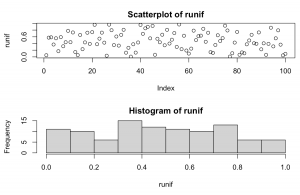
Explanation: Takes 100 random samples from between a minimum value of 0 and maximum value of 1. The formula defaults to between 0 and 1, but could assume any number combination really.
Simulate data using a Normal (Gaussian) distribution
set.seed(1234)
normal <- rnorm(100, 0, 1)
par(mfrow=c(2,1))
plot(normal, main = "Scatterplot of normal")
hist(normal)
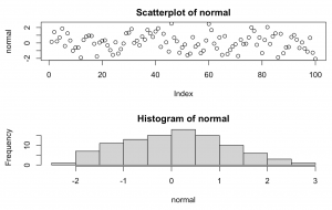
Explanation: Takes 100 random samples from a classic bell curve with mean = 0 and standard deviation = 1. This could easily be adjusted to reflect an age related study where mean = 25, sd = 2.5, and we had 150 participants.
It’s also pretty easy to generate a ‘normally’ distributed series of numbers that is also skewed (see further for instance package fGarch that includes a ‘xi’ parameter that introduces skew.
However, it’s also easy to head over to a naturally skewed distribution and just sample from that one instead, such as the Gamma distribution below.
Simulate data using a Gamma distribution
The Gamma distribution offers several alternatives depending upon the shape parameter chosen, with lower numbers i.e. =1 being more right skewed, while higher numbers i.e. =10 are less right skewed;
set.seed(1234)
gamma <- rgamma(n=100, shape = 5)
par(mfrow=c(2,1))
plot(gamma, main = "Scatterplot of Gamma")
hist(gamma)
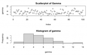
Explanation: Takes 100 random samples from a Gamma distribution with shape = 5. This is a right skewed Gamma distribution which peaks around values = 2-4.
Simulate data using a Exponential distribution
The exponential distribution is a particular example of the Gamma distribution above. It tends to characterise a pattern of time decay e.g. (rates of decay of particular chemical elements). The exponential distribution is also very close to a Gamma distribution of shape = 1.
set.seed(1234)
exp <- rexp(n = 100, rate = 0.5)
par(mfrow=c(2,1))
plot(exp, main = "Scatterplot of Exponential")
hist(exp)
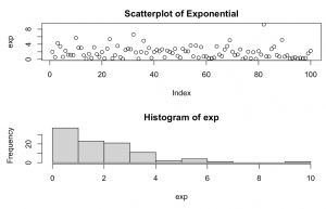
Explanation: takes 100 random samples from an Exponential distribution with each successive observation one half of the preceding one. Thus, as the rate decreases, the steepness of the curve increases.
Simulate data using a Binomial distribution
This distribution is a an example of a discrete distribution, as it can only accept certain values. In the code below, we’ve instructed it to sample from only two values: 0 and 1 (via the size=n sub-statement). The prob=x sub-statement is the probability of success, here instructed to be a 50/50 chance of success.
set.seed(1234)
binomial <- rbinom(n = 100, size = 1, prob = 0.5)
par(mfrow=c(2,1))
plot(binomial, main = "Scatterplot of Binomial")
hist(binomial)
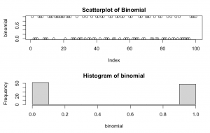
Explanation: takes 100 random samples from a binomial distribution with only 2 values, zero and one and a likelihood of success of 50%.
Simulate data using a Poisson distribution
The Poisson distribution is best used to model count data that is relatively constant over time, such as the number of times a particular number comes up on a dice, or the number of cars that run a red light within a certain interval of time. It is kind of a curious cross between binomial and an exponential distributions, in that it reflects the likelihood of a particular event occurring with a mean value known before hand. This mean value lends a degree of skew to the distribution as seen in the right skew below.
set.seed(1234)
poisson <- rpoisson(n = 100, lambda = 1)
par(mfrow=c(2,1))
plot(poisson, main = "Scatterplot of Poisson")
hist(poisson)
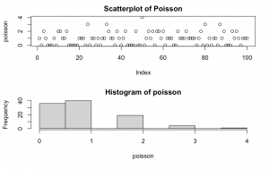
Explanation: takes 100 random samples from a Poisson distribution with mean = 1.
Conclusion
Hopefully, this post gives you a one-stop shop to access a range of probability distributions. In particular, I hope I’ve explained how to generate a series of random numbers that follows the shape of particular probability distributions.
This can come in very handy when you’re trying to generate a dataset for an lesson, for your own fun, to simulate a study, or even to perform a power analysis.
0 Comments